Create a PivotTable in Excel for Windows
Create a PivotTable in Excel for Windows
Select the cells you want to create a PivotTable from.
Note: Your data should be organized in columns with a single header row.
Select Insert > PivotTable.
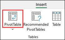
This will create a PivotTable based on an existing table or range.
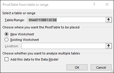
Note: Selecting Add this data to the Data Model will add the table or range being used for this PivotTable into the workbook’s Data Model. Learn more.
Choose where you want the PivotTable report to be placed. Select New Worksheet to place the PivotTable in a new worksheet or Existing Worksheet and select where you want the new PivotTable to appear.
Click OK
PivotTables from other sources
By clicking the down arrow on the button, you can select from other possible sources for your PivotTable. In addition to using an existing table or range, there are three other sources you can select from to populate your PivotTable.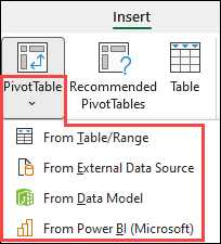
Note: Depending on your organization's IT settings you might see your organization's name included in the button. For example, "From Power BI (Microsoft)"
From External Data Source
From Data Model
Use this option if your workbook contains a Data Model, and you want to create a PivotTable from multiple Tables, enhance the PivotTable with custom measures, or are working with very large datasets. 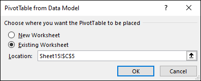
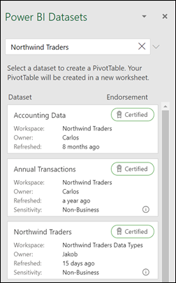
From Power BI
Use this option if your organization uses Power BI and you want to discover and connect to endorsed cloud datasets you have access to.
Building out your PivotTable
To add a field to your PivotTable, select the field name checkbox in the PivotTables Fields pane.
Note: Selected fields are added to their default areas: non-numeric fields are added to Rows, date and time hierarchies are added to Columns, and numeric fields are added to Values.
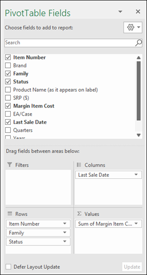
To move a field from one area to another, drag the field to the target area.
Create a PivotChart
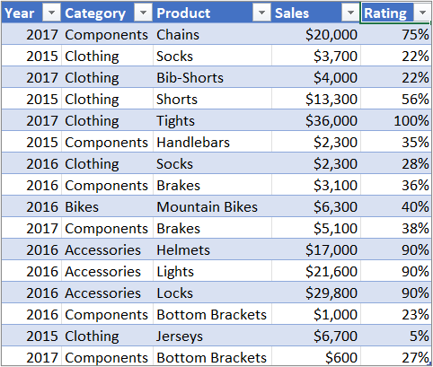
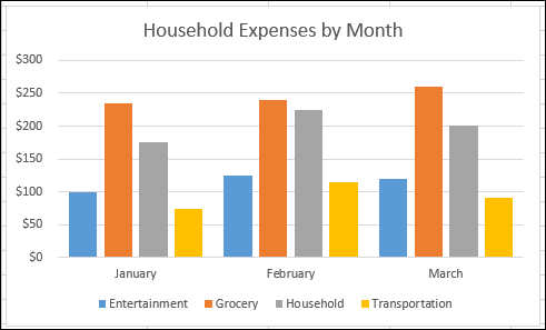
Sometimes it's hard to see the big picture when your raw data hasn’t been summarized. Your first instinct may be to create a PivotTable, but not everyone can look at numbers in a table and quickly see what's going on. PivotCharts are a great way to add data visualizations to your data.
Household expense data | Corresponding PivotChart |
|
|
Create a PivotChart
Select a cell in your table.
Select Insert > PivotChart
 .
.Select OK.
Create a chart from a PivotTable
Select a cell in your table.
Select PivotTable Tools > Analyze > PivotChart
.Select a chart.
Select OK.
Use slicers to filter data
Slicers provide buttons that you can click to filter tables, or PivotTables. In addition to quick filtering, slicers also indicate the current filtering state, which makes it easy to understand what exactly is currently displayed.
You can use a slicer to filter data in a table or PivotTable with ease.
Create a slicer to filter data
Click anywhere in the table or PivotTable.
On the Home tab, go to Insert > Slicer.

In the Insert Slicers dialog box, select the check boxes for the fields you want to display, then select OK.
A slicer will be created for every field that you selected. Clicking any of the slicer buttons will automatically apply that filter to the linked table or PivotTable.
Notes:
To select more than one item, hold Ctrl, and then select the items that you want to show.
To clear a slicer's filters, select Clear Filter
 in the slicer.
You can adjust your slicer preferences in the Slicer tab (in newer versions of Excel), or the Design tab (Excel 2016 and older versions) on the ribbon.
Note: Select and hold the corner of a slicer to adjust and resize it.
If you want to connect a slicer to more than one PivotTable, go to Slicer > Report Connections > check the PivotTables to include, then select OK.
Note: Slicers can only be connected to PivotTables that share the same data source.
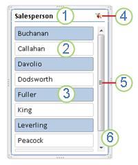
Slicer components
A slicer typically displays the following components:
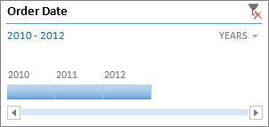
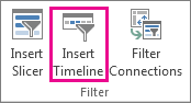
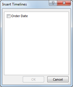
| 1. A slicer header indicates the category of the items in the slicer. 2. A filtering button that is not selected indicates that the item is not included in the filter. 3. A filtering button that is selected indicates that the item is included in the filter. 4. A Clear Filter button removes the filter by selecting all items in the slicer. 5. A scroll bar enables scrolling when there are more items than are currently visible in the slicer. 6. Border moving and resizing controls allow you to change the size and location of the slicer. Create a PivotTable timeline to filter datesInstead of adjusting filters to show dates, you can use a PivotTable Timeline—a dynamic filter option that lets you easily filter by date/time, and zoom in on the period you want with a slider control. Click Analyze > Insert Timeline to add one to your worksheet.
Much like a slicer for filtering data, you can insert a Timeline one time, and then keep it with your PivotTable to change the range of time whenever you like.
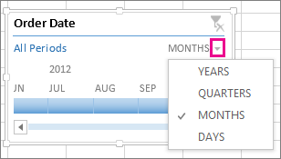
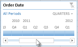
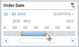
Use a Timeline to filter by time periodWith your Timeline in place, you’re ready to filter by a time period in one of four time levels (years, quarters, months, or days).
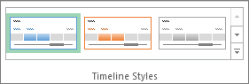
Use a Timeline with multiple PivotTablesProvided your PivotTables are using the same data source, you can use a single Timeline to filter multiple PivotTables. Select the Timeline, then on the ribbon, go to Options > Report Connections, and select the PivotTables you want to include. Clear a timelineTo clear a timeline, click the Clear Filter button Tip: If you want to combine slicers with a timeline to filter the same date field, you can do that by checking the Allow multiple filters per field box in the PivotTable Options dialog box (PivotTable Tools > Analyze > Options > Totals & Filters tab). Customize a timelineWhen a timeline covers your PivotTable data, you can move it to a better location and change its size. You can also change the timeline style, which may be useful if you have more than one timeline.
|
 .
.
Calculate values in a PivotTable
In PivotTables, you can use summary functions in value fields to combine values from the underlying source data. If summary functions and custom calculations do not provide the results that you want, you can create your own formulas in calculated fields and calculated items. For example, you could add a calculated item with the formula for the sales commission, which could be different for each region. The PivotTable would then automatically include the commission in the subtotals and grand totals.
Create formulas in a PivotTable
Important: You cannot create formulas in a PivotTable that is connected to an Online Analytical Processing (OLAP) data source.
Before you start, decide whether you want a calculated field or a calculated item within a field. Use a calculated field when you want to use the data from another field in your formula. Use a calculated item when you want your formula to use data from one or more specific items within a field.
For calculated items, you can enter different formulas cell by cell. For example, if a calculated item named OrangeCounty has a formula of =Oranges * .25 across all months, you can change the formula to =Oranges *.5 for June, July, and August.
If you have multiple calculated items or formulas, you can adjust the order of calculation.
Add a calculated field
Click the PivotTable.
This displays the PivotTable Tools, adding the Analyze and Design tabs.
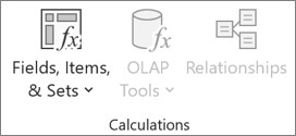
On the Analyze tab, in the Calculations group, click Fields, Items, & Sets, and then click Calculated Field.
In the Name box, type a name for the field.
In the Formula box, enter the formula for the field.
To use the data from another field in the formula, click the field in the Fields box, and then click Insert Field. For example, to calculate a 15% commission on each value in the Sales field, you could enter = Sales * 15%.
Click Add.
Add a calculated item to a field
Click the PivotTable.
This displays the PivotTable Tools, adding the Analyze and Design tabs.
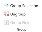
If items in the field are grouped, on the Analyze tab, in the Group group, click Ungroup.
Click the field where you want to add the calculated item.
On the Analyze tab, in the Calculations group, click Fields, Items, & Sets, and then click Calculated Item.
In the Name box, type a name for the calculated item.
In the Formula box, enter the formula for the item.
To use the data from an item in the formula, click the item in the Items list, and then click Insert Item (the item must be from the same field as the calculated item).
Click Add.
Enter different formulas cell by cell for calculated items
Click a cell for which you want to change the formula.
To change the formula for several cells, hold down CTRL and click the additional cells.
In the formula bar, type the changes to the formula.
Adjust the order of calculation for multiple calculated items or formulas
Click the PivotTable.
This displays the PivotTable Tools, adding the Analyze and Design tabs.
On the Analyze tab, in the Calculations group, click Fields, Items, & Sets, and then click Solve Order.
Click a formula, and then click Move Up or Move Down.
Continue until the formulas are in the order that you want them to be calculated.
View all formulas that are used in a PivotTable
You can display a list of all the formulas that are used in the current PivotTable.
Click the PivotTable.
This displays the PivotTable Tools, adding the Analyze and Design tabs.
On theAnalyze tab, in the Calculations group, click Fields, Items, & Sets, and then click List Formulas.
Edit a PivotTable formula
Before you edit a formula, determine whether that formula is in a calculated field or a calculated item. If the formula is in a calculated item, also determine whether the formula is the only one for the calculated item.
For calculated items, you can edit individual formulas for specific cells of a calculated item. For example, if a calculated item named OrangeCalc has a formula of =Oranges * .25 across all months, you can change the formula to =Oranges *.5 for June, July, and August.
Determine whether a formula is in a calculated field or a calculated item
Click the PivotTable.
This displays the PivotTable Tools, adding the Analyze and Design tabs.
On the Analyze tab, in the Calculations group, click Fields, Items, & Sets, and then click List Formulas.
In the list of formulas, find the formula that you want to change listed under Calculated Field or Calculated Item.
When there are multiple formulas for a calculated item, the default formula that was entered when the item was created has the calculated item name in column B. For additional formulas for a calculated item, column B contains both the calculated item name and the names of intersecting items.For example, you might have a default formula for a calculated item named MyItem, and another formula for this item identified as MyItem January Sales. In the PivotTable, you would find this formula in the Sales cell for the MyItem row and January column.
Continue by using one of the following editing methods.
Edit a calculated field formula
Click the PivotTable.
This displays the PivotTable Tools, adding the Analyze and Design tabs.
On the Analyze tab, in the Calculations group, click Fields, Items, & Sets, and then click Calculated Field.
In the Name box, select the calculated field for which you want to change the formula.
In the Formula box, edit the formula.
Click Modify.
Edit a single formula for a calculated item
Click the field that contains the calculated item.
On the Analyze tab, in the Calculations group, click Fields, Items, & Sets, and then click Calculated Item.
In the Name box, select the calculated item.
In the Formula box, edit the formula.
Click Modify.
Edit an individual formula for a specific cell of a calculated item
Click a cell for which you want to change the formula.
To change the formula for several cells, hold down CTRL and click the additional cells.
In the formula bar, type the changes to the formula.
Tip: If you have multiple calculated items or formulas, you can adjust the order of calculation. For more information, see Adjust the order of calculation for multiple calculated items or formulas.
Delete a PivotTable formula
Note: Deleting a PivotTable formula removes it permanently. If you do not want to remove a formula permanently, you can hide the field or item instead by dragging it out of the PivotTable.
Determine whether the formula is in a calculated field or a calculated item.
Calculated fields appear in the PivotTable Field List. Calculated items appear as items within other fields.
Do one of the following:
To delete a calculated field, click anywhere in the PivotTable.
To delete a calculated item, in the PivotTable, click the field that contains the item that you want to delete.
This displays the PivotTable Tools, adding the Analyze and Design tabs.
On the Analyze tab, in the Calculations group, click Fields, Items, & Sets, and then click Calculated Field or Calculated Item.
In the Name box, select the field or item that you want to delete.
Click Delete.
Use multiple tables to create a PivotTable
PivotTables are great for analyzing and reporting on your data. And when your data happens to be relational—meaning it's stored in separate tables you can bring together on common values—you can build a PivotTable like this in minutes:
What’s different about this PivotTable? Notice how the Field List on the right shows not just one but a collection of tables. Each of these tables contain fields you can combine in a single PivotTable to slice your data in multiple ways. No manual formatting or data preparation is necessary. You can immediately build a PivotTable based on related tables as soon as you import the data.
To get multiple tables into the PivotTable Field List:
Import from a relational database, like Microsoft SQL Server, Oracle, or Microsoft Access. You can import multiple tables at the same time.
Import multiple tables from other data sources including text files, data feeds, Excel worksheet data, and more. You can add these tables to the Data Model in Excel, create relationships between them, and then use the Data Model to create your PivotTable.
Here's how you'd import multiple tables from a SQL Server database.
Make sure you know the server name, database name, and which credentials to use when connecting to SQL Server. Your database administrator can provide the necessary information.
Click Data > Get External Data > From Other Sources > From SQL Server.
In the Server Name box, enter the network computer name of the computer that runs SQL Server.
In the Log on credentials box, click Use Windows Authentication if you're connecting as yourself. Otherwise, enter the username and password provided by the database administrator.
Press Enter and, in the Select Database and Table box, choose the database you want, then click Enable selection of multiple tables.
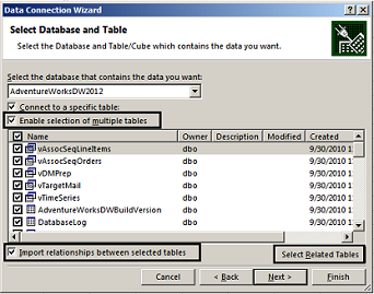
If you know exactly which tables you want to work with, manually choose them. Otherwise, pick one or two, then click Select Related Tables to auto-select tables that are related to those you selected.
If the Import relationships between selected tables box is checked, keep it that way to allow Excel to recreate equivalent table relationships in the workbook.
Click Finish.
In the Import Data dialog box, choose PivotTable Report.
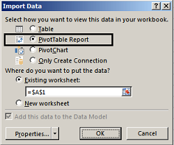
Click OK to start the import and populate the Field List.
Notice that the Field List contains multiple tables. These are all of the tables that you selected during import. You can expand and collapse each table to view its fields. As long as the tables are related, you can create your PivotTable by dragging fields from any table to the VALUES, ROWS, or COLUMNS areas.
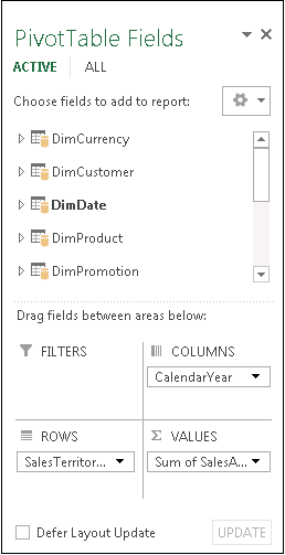
Drag numeric fields to the VALUES area. For example, if you are using an Adventure Works sample database, you might drag SalesAmount from the FactInternetSales table.
Drag date or territory fields to the ROWS or COLUMNS area to analyze sales by date or territory.
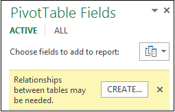
Sometimes you need to create a relationship between two tables before you can use them in a PivotTable. If you get a message indicating a relationship is needed, click Create to get started.
If you're working with other types of databases:
To use other relational databases, such as Oracle, you might need to install additional client software. Check with your database administrator to find out if this is required.
You can import multiple tables from Access. See Tutorial: Import Data into Excel, and Create a Data Model for details.
Import tables from other sources
In addition to SQL Server, you can import from a number of other relational databases:
Relational databases are not the only data source that lets you work with multiple tables in a PivotTable Field List. You can use tables in your workbook, or import data feeds that you then integrate with other tables of data in your workbook. To make all this unrelated data work together, you’ll need to add each table to the Data Model, and then create relationships between the tables using matching field values.
Use the Data Model to create a new PivotTable
Perhaps you’ve created relationships between tables in the Data Model, and are now ready to use this data in your analysis. Here's how you build a new PivotTable or PivotChart using the Data Model in your workbook.
Click any cell on the worksheet.
Click Insert > PivotTable.

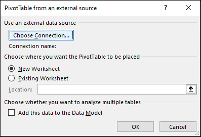
In the Create PivotTable dialog box, click From External Data Source.
Click Choose Connection.
On the Tables tab, in This Workbook Data Model, select Tables in Workbook Data Model.
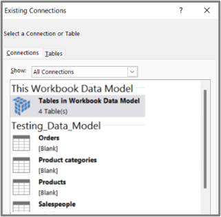
Click Open, and then click OK to show a Field List containing all the tables in the Data Model.
Use the Field List to arrange fields in a PivotTable
After you create a PivotTable, you'll see the Field List. You can change the design of the PivotTable by adding and arranging its fields. If you want to sort or filter the columns of data shown in the PivotTable, see Sort data in a PivotTable and Filter data in a PivotTable.
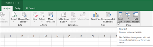
The Field List should appear when you click anywhere in the PivotTable. If you click inside the PivotTable but don't see the Field List, open it by clicking anywhere in the PivotTable. Then, show the PivotTable Tools on the ribbon and click Analyze> Field List.
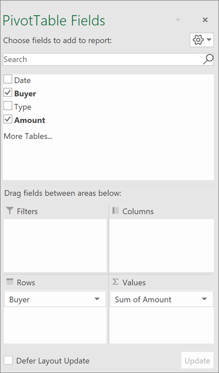
The Field List has a field section in which you pick the fields you want to show in your PivotTable, and the Areas section (at the bottom) in which you can arrange those fields the way you want.
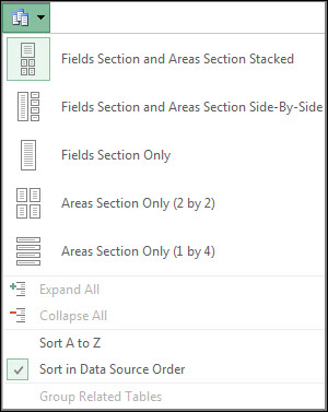
Tip: If you want to change how sections are shown in the Field List, click the Tools button  and then pick the layout you want.
Add and rearrange fields in the Field List
Use the field section of the Field List to add fields to your PivotTable, by checking the box next to field names to place those fields in the default area of the Field List.
NOTE: Typically, nonnumeric fields are added to the Rows area, numeric fields are added to the Values area, and Online Analytical Processing (OLAP) date and time hierarchies are added to the Columns area.
Use the areas section (at the bottom) of the Field List to rearrange fields the way you want by dragging them between the four areas.
Fields that you place in different areas are shown in the PivotTable as follows:
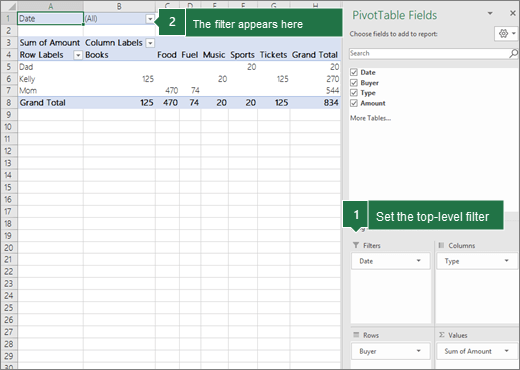
Filters area fields are shown as top-level report filters above the PivotTable, like this:
Columns area fields are shown as Column Labels at the top of the PivotTable, like this:

Depending on the hierarchy of the fields, columns may be nested inside columns that are higher in position.
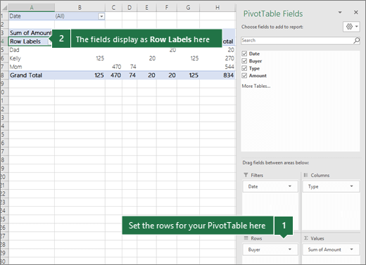
Rows area fields are shown as Row Labels on the left side of the PivotTable, like this:
Depending on the hierarchy of the fields, rows may be nested inside rows that are higher in position.
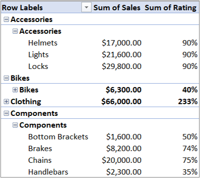
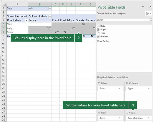
Values area fields are shown as summarized numeric values in the PivotTable, like this:
If you have more than one field in an area, you can rearrange the order by dragging the fields into the precise position you want. To delete a field from the PivotTable, drag the field out of its areas section.


Comments
Post a Comment