What is VLOOKUP in Excel
- Get link
- X
- Other Apps
What is VLOOKUP in Excel and How to use it?


In this data-driven world, one needs various tools in order to manage data. Data in real-time is huge and fetching details regarding some particular piece of data would definitely be a tiring task but with VLOOKUP in Excel, this task can be achieved with a single line of command. In this article, you will be learning about one of the important Excel functions i.e the VLOOKUP Function.
Before moving on, let’s take a quick look at all the topics that are discussed over here:
- What is VLOOKUP in Excel?
- How does it work?
- Exact Match
- Approximate Match
- First Match
- Case Sensitivity
- Errors
- Two-way Lookup
- Using Wildcards
- Multiple Lookup tables
What is VLOOKUP in Excel?
In Excel, VLOOKUP is a built-in function that is used to lookup and fetch specific data from an excel sheet. V stands for Vertical and in order to use the VLOOKUP function in Excel, the data must be arranged vertically. This function comes in very handy when you have a huge amount of data and would be practically impossible to manually search for some specific data.
How does it work?
The VLOOKUP function takes a value i.e the lookup value and starts to search for it in the leftmost column. When the first occurrence of the lookup value is found, it starts to move right in that row and returns a value from the column that you specify. This function can be used to return both exact as well as approximate matches (The default match is an approximate match).
Syntax:
The syntax of this function is as follows:
VLOOKUP(lookup_value, table_array, col_index_num, [range_lookup])
- lookup_value is the value to be looked out for in the first column of the given table
- table_index is the table from which the data is to be fetched
- col_index_num is the column from which the value is to be fetched
- range_lookup is a logical value that determines if the lookup value should be a perfect match or an approximate match (TRUE will find the closest match; FALSE checks for exact match)
Exact Match:
When you want the VLOOKUP function to look for an exact match of the lookup value, you will have to set the range_lookup value to FALSE. Take a look at the following example which is a table consisting of employee details:
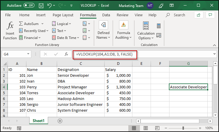
In case you want to look for the designation of any of these employees, you can do as follows:
- Select the cell where you want to display the output and then type a “=” sign
- Use the VLOOKUP function and supply the lookup_value (Here, it will be the employee ID)
- Then pass in the other parameters i.e the table_array, col_index_num and set the range_lookup value to FALSE
- Therefore, the function and its parameters will be: =VLOOKUP(104, A1: D8, 3, FALSE)
The VLOOKUP function starts to look for the employee ID 104 and then moves towards the right in the row where the value is found. It goes on till the col_index_num and returns the value present at that position.
Approximate Match:
This feature of the VLOOKUP function allows you to retrieve values even when you do not have an exact match for the loopup_value. As mentioned earlier, in order to make VLOOKUP look for an approximate match, you will need to set range_lookup value to TRUE. Take a look at the following example where the marks are mapped along with their grades and the class to which they belong.
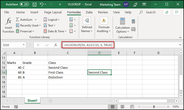
- Just like how you did for an exact match, follow the same steps
- In place of the range_lookup value, use TRUE instead of FALSE
- Therefore, the function along with its parameters will be: =VLOOKUP(55, A12: C15, 3, TRUE)
In a table that is sorted in the ascending order, VLOOKUP starts to look for an approximate match and stops at the next largest value that is smaller than the lookup value that you have entered. It then moves right in that row and returns the value from the specified column. In the above example, the lookup value is 55 and the next largest lookup value in the first column is 40. Therefore, the output is Second Class.
First Match:
In case you have a table that consists of multiple lookup values, VLOOKUP stops at the first match of it and retrieves a value from that row in the specified column.
Take a look at the image below:
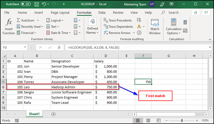
The ID 105 is repeated and when the lookup value is specified as 105, VLOOKUP has returned the value from the row that has the first occurrence of the lookup value.
Case Sensitivity:
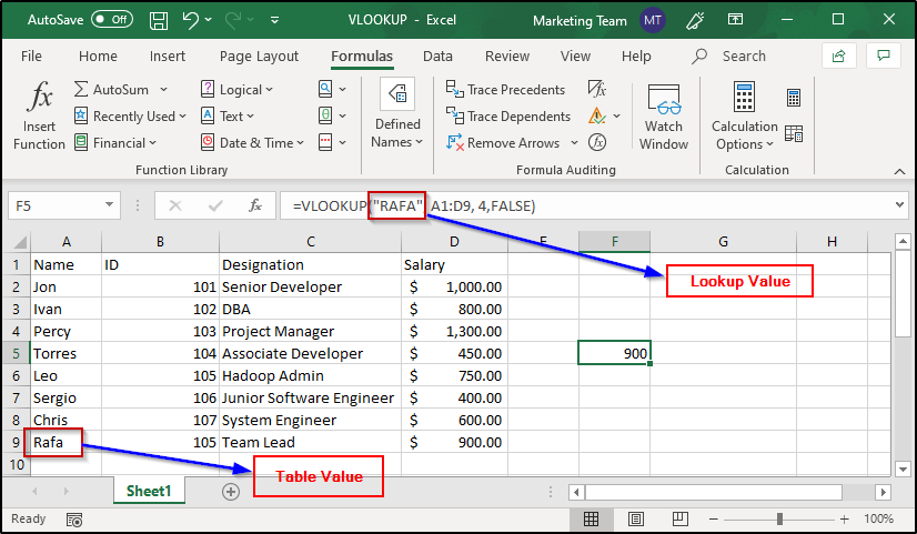
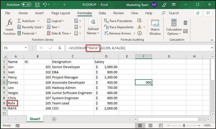
VLOOKUP function is case insensitive. In case you have a lookup value that in upper case and the value present in the table is small, VLOOKUP will still fetch the value from the row in which the value is present. Take a look at the image below:

MSBI Certification Training Course
- Instructor-led Sessions
- Real-life Case Studies
- Assignments
- Lifetime Access
As you can see, the value that I have specified as a parameter is “RAFA” whereas the value present in the table is “Rafa” but VLOOKUP has still returned the specified value. If you have an exact match even with the case, VLOOKUP will still return the first match of the lookup value irrespective of the case used. Take a look at the image below:
Errors:
It is natural to encounter errors whenever we make use of functions. Similarly, you can encounter errors when using VLOOKUP function as well and some of the common errors are:
- #NAME
- #N/A
- #REF
- #VALUE
#NAME Error:
This error basically is to inform you that you have made some mistake in the syntax. To avoid syntactical errors, it’s better to use the Function Wizard provided by Excel for every function. The Function Wizard helps you with information regarding every parameter and the type of values that you need to enter. Take a look at the image below:
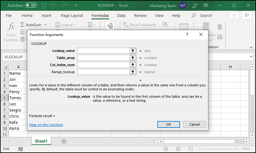
As you can see, the Function Wizard informs you to enter any type of value in place of the lookup_value parameter and also gives a brief description of the same. Similarly, when you select the other parameters, you will see information regarding them as well.
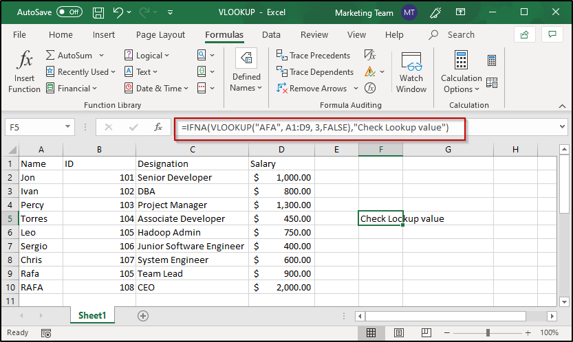
#N/A Error:
This error is returned in case no match is found for the given lookup value. For example, if I enter “AFA” instead of “RAFA”, I will get #N/A error.

In order to define some error message for the above two errors, you can make use of the IFNA function. For example:
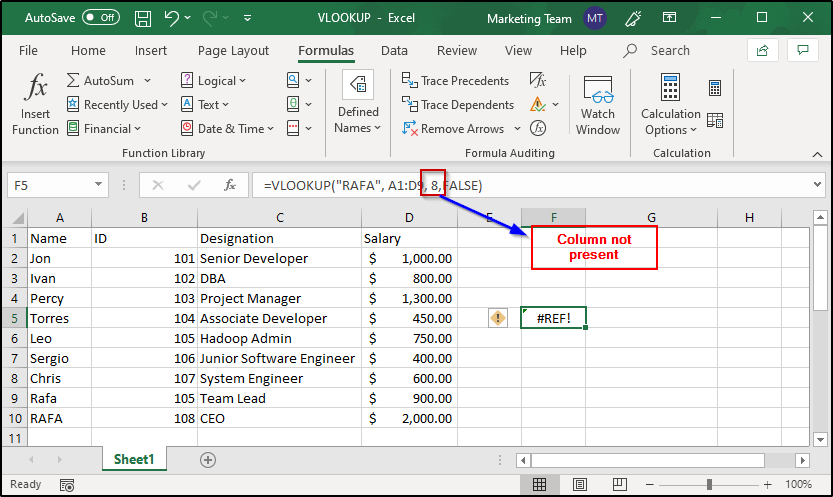
#REF Error:
This error is encountered when you give reference to a column that is not available in the table.
#VALUE Error:
This error is encountered when you place wrong values to the parameters or miss some compulsory parameters.

Two-way Lookup:
Two-way lookup refers to fetching a value from a two-dimensional table from any cell of the referenced table. In order to perform a two-way lookup using VLOOKUP, you will need to use the MATCH function along with it.
- Get link
- X
- Other Apps


Comments
Post a Comment