VLOOKUP in Excel
VLOOKUP Function (Table of contents)
Introduction to VLOOKUP Function in Excel
Vlookup function is used to lookup the value with a reference cell and fetch the value from the selected lookup table array and is quite useful and one of the most widely used excel functions. We can use a table or single column to lookup the value. And all the lookup can be done in a vertical zone or with columns only.
VLOOKUP Formula in Excel:
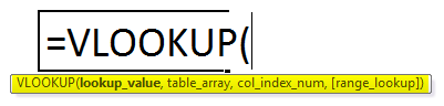
The vlookup function uses of the arguments:-
There are four arguments in the vlookup function, which is below mention:
- Lookup value (required argument) is the value that we want to look up in a table column. Where you want or get the value from another table.
- Table array (required argument) – it is the data array that is to be searched. The vlookup function searches in the left-most column of this array. We can say that this is a matching table.
- Column index number (required argument) – an integer specifying the column number of the supplied table array that you want to return a value from. If you are only using it for data matching, you can put 1, but if you want to get a value from another column to match the lookup value, you need to put column no from matching column no.
- Range lookup (optional argument) defines what this function should return if it does not find an exact match to the lookup value. The argument can be set to true or false, which means:
- True – approximate match; if an exact match is not found, use the closest match below the lookup value.
- False – exact match; if an exact match is not found, then it will return an error.
- We can also use 0 for false and 1 for true matching.
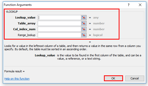
Steps for Using VLOOKUP Function
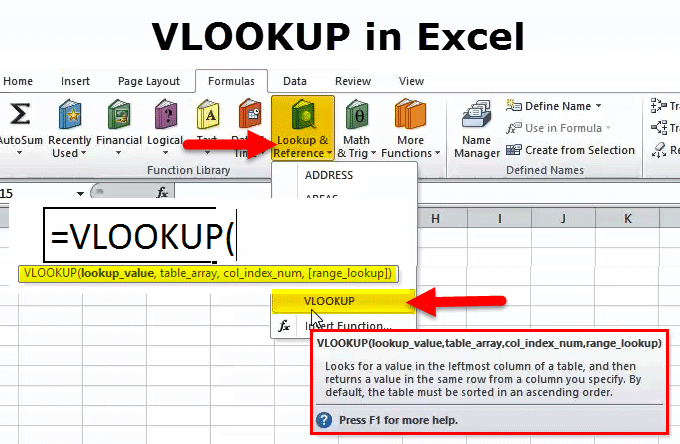
- Click on formula tab > lookup & reference > click on vlookup.
- Also, click on the function icon, then manually write and search the formula.
- We get a new function window showing in the below mention pictures.
- Then we have to enter the details as shown in the picture.
- Put the lookup value where you want to match from one table to another table value.
- You need to put the table array, which is another table value.
- Put the col index number for another table vertical value which is a need.
- Rage lookup false for exact match and true for an approximate match.
- You can also use 0 for an exact match and 1 for an approximate match.
Shortcut for using the Formula
Click on a cell where you want to result in value then put the formula as below mention
= vlookup (lookup value, table range, column index) > enter
An explanation for VLOOKUP Function:
This function helps you to locate specific information in your spreadsheet. When the user uses the vlookup function for finding specific information in an MS Excel spreadsheet, each matching information is displayed in the same row but in the next column. This function performs a vertical lookup by searching for a value in the first column of a table and returning the value in the same row in the index number position.
We can also use one sheet to another sheet and one workbook to another workbook also.
How to Use VLOOKUP in Excel?
Vlookup function is very simple and easy to use. Let us understand the working of vlookup. Below mention are the details using the formulas.
Example #1 – Exact Match
To search for an exact match, you put false in the last argument.
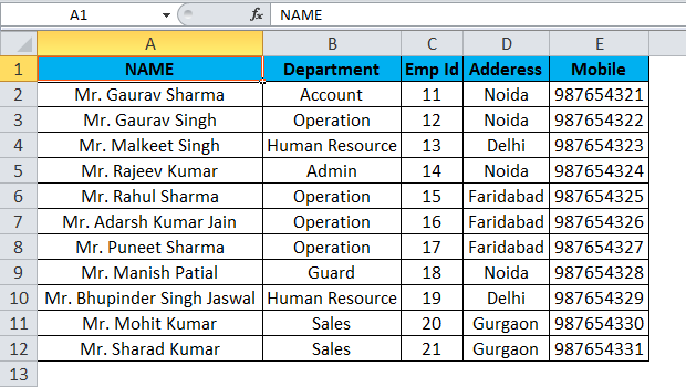
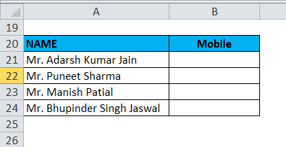
As mentioned in table b, there is all employee information like department, employee id, address, mobile no, etc. So you can suppose as array table or master table data. And you have another table where required only contact no of the employee. So as the employee name is a unique column, then the employee names a lookup value in a table where you want to get a result.
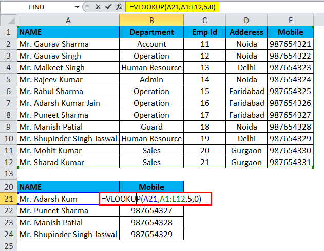
Master data table b, as above showing, is a table array, and in master data, you can see that mobile no column is on the 5 number column index. So then we need to put the 0 for exact matching or 1 for false matching.
You can see the result here:
Formula: – “=vlookup(a21,a1:e12,5,0)”
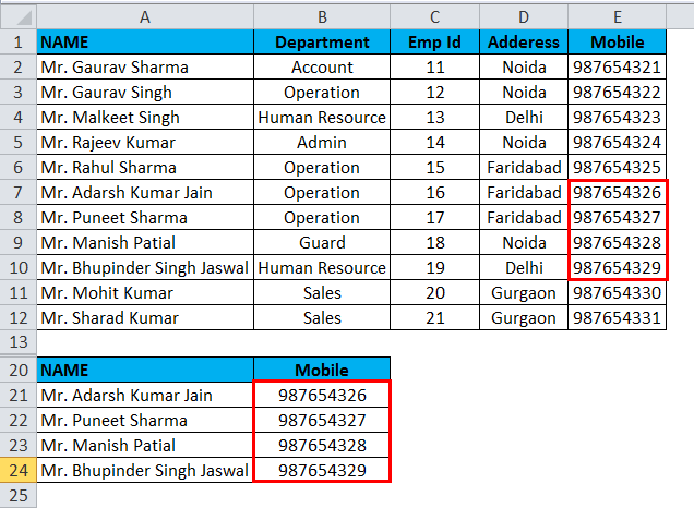
We can see that in a table, all values are matching the exact value.
Example #2 – Approximate Match
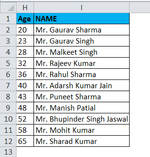
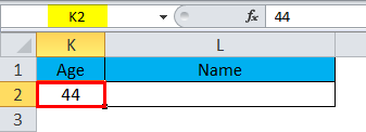
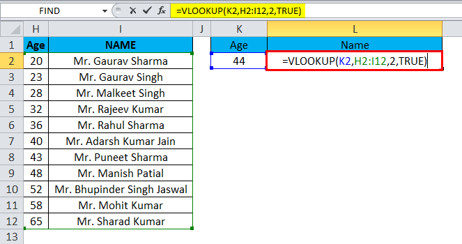
As above showing in the picture in the H column, there is employee age mention and column I employee name. You can take this as an array or master table. Now I want to put the age value in k2; then we get the employee name which is approximate age as given in k2 age value as showing below mention pictures.
So lets we check the formula now.
“=vlookup(k2,h2:i12,2,true)”
Then we can get the approximate matching value.
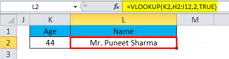
As you see, the formula returns Mr. Puneet Sharma, whose age is 43, while we also have Mr. Manish Patil, that age is 48, but 43 is much closer to 44 than 48. So, why does it return Mr. Puneet? Because vlookup with approximate match retrieves the closest value that is less than the lookup value.

4.9 (10,456 ratings)
₹1999
View Course
Things to Remember
- The vlookup function returns result in any data type such as a string, numeric, date, etc.
- If you specify false for the approximate match parameter and no exact match is found, then the vlookup function will return #n/a.
- If you specify true for the approximate match parameter and no exact match is found, then the next smaller value is returned.
- If the index number is less than 1, the vlookup function will return the #value!.
If the index number is greater than the number of columns in the table, the vlookup function will return #ref!
Introduction to VLOOKUP Examples in Excel
This article covers one of the most helpful features, which is VLOOKUP. Simultaneously it is one of the most complex and less understood functions. In this article, we will demystify VLOOKUP with a few examples.
Examples of VLOOKUP in Excel
VLOOKUP in Excel is very simple and easy to use. Let’s understand how to use the VLOOKUP in Excel with some examples.
Example #1 – Exact Match (False or 0)
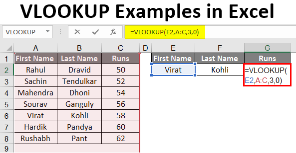
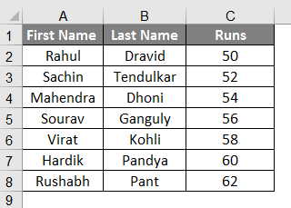
Here for this example, let’s make a table to use this formula; suppose we have the data of students as shown in the image below.
In cell F2, we are using VLOOKUP Formula. We have made the table; by using Vlookup, we will find the Last name of the person from their first name; all the data has to be available in the table which we are providing the range to find the answer within (A:C in this case).
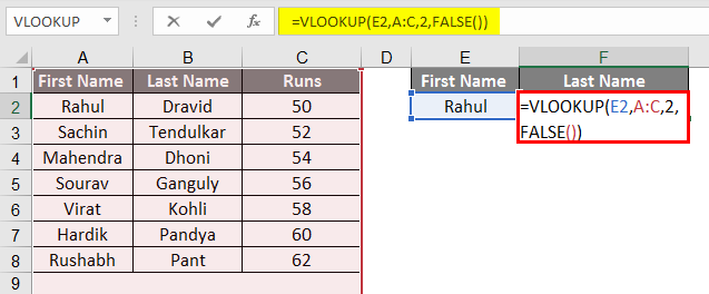
- We can select the table too instead of the entire row; In the formula, you can see written 2 before False as a column indicator because we want data to be retrieved from column # 2 from the selected range.
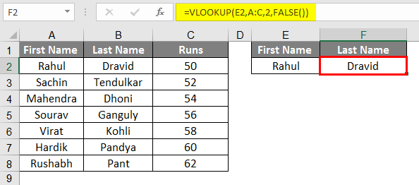
- Here when we place data in E3, which is the first name from our given table, the formula will give us the Last Name.
- When we enter the first name from a table, we are supposed to get the formula’s last name.
- From the Image above, we can see that by writing the name Rahul in the column, we got Dravid the second name according to the table on the left.
- Now we can also widen the data from a single data available, so by just filling the First Name, we will have the Last name of the person and the runs scored by that person.
- So let’s add the third column on the right side, “Runs”.
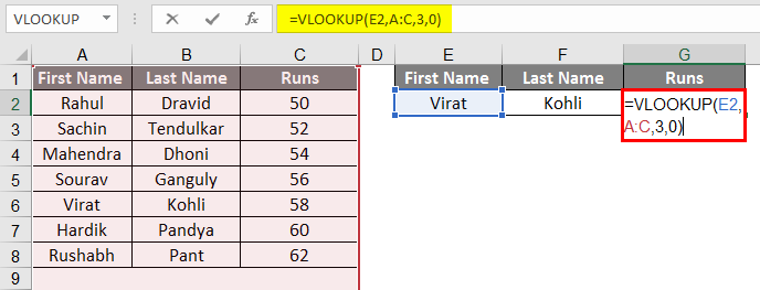
- After applying VLOOKUP Formula, the result is shown below.
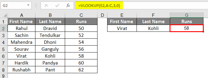
- We can see that just from the first name, we have got the last name and the runs scored by that student; If we retrieve runs from the last name column, it will be called chained Vlookup.
- Here you can see we have written 3 as we want the data of column #3 from the range we have selected.
- Here we have used False OR 0, which means it is matching the absolute value, so by applying even extra space to our first name, it will show the #N/A means data not matching.
Example #2 – Approximate Match (True or 1)
- If we apply the same formula with True or 1 instead of False or 0, we will not have to worry about providing the exact data to the system.
- This formula will provide the same results, but it will start to look from top to bottom and provides the value with the most approx match.
- So even after you make some spelling mistake or a grammatical error in our case, you don’t need to worry, as it will find the most matched data and provides the result of mostly matched.
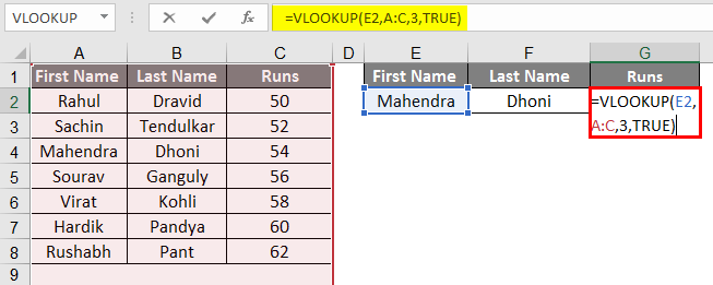
- After applying VLOOKUP Formula, the results are shown below.
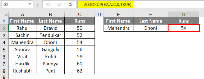
- In our example, we have written Mahendra in the first name, and still, we are getting the result correctly; this can be a bit complicated while you’re playing with the words but more comfortable while you’re working with Numbers.
- Suppose we have Numeric data instead of the name or word or alphabetical; we can do this more precisely and with more authentic logic.
- It seems pretty useless as here we are dealing with small data, but it is very useful while dealing with large data.
Example #3 – Vlookup from a Different Sheet
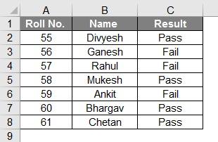
- Vlookup from a different sheet is very much similar to the Vlookup from the same sheet, so here we have changed in the ranges, as here we have different worksheets.
- We have a table in sheet number 2 as per the following image; we will find the result of this student in sheet number 3 from their roll nos.
- As you can see, the image on the right side is of another sheet, sheet number 3.
- Apply the VLOOKUP Formula in Column B.
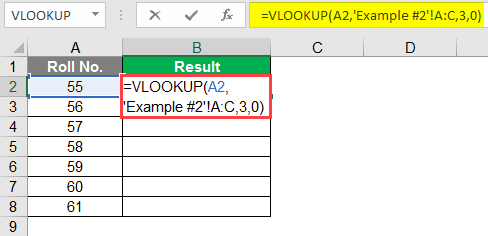
- After applying VLOOKUP Formula, the result is shown below.
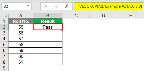
- Drag down the formula for the next cell. So the output will be as below.
- From the above images, you can see that the range of the formula has been indicated with ‘Example#2′ as the data we needed will be retrieved from Example #2 and column #3. So as a column indicator, we have written 3, and then 0 means False as we want exact data match.
- As you can see from the below image, we have successfully retired the entire data from Example #2 to Sheet # 3.
- You can see from the above image, after getting the value in the first row, we can drag the same and get to throughout data against the given roll nos if it is available in the given table.
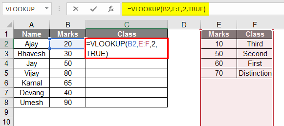
Example #4 – Class Using Approx Match
- To define class from the marks, we can use an approx match to define the class against the Marks.
After using the VLOOKUP formula, the result is shown below
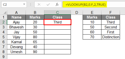
- As per the above image, you can see that we have made a table of students with marks to identify their class; we have made another table that will act as the key,
- But make sure that the marks in the cell have to be in ascending order.
- So in the given data, the formula converts the marks into a grade from the class table or “Key” table.
- Drag the same formula from cell C2 to C9.
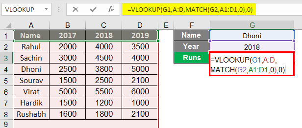
Example #5 – Dual Lookup Using Match function
- The Match function is used when we need to lookup two-way data; here, from the above table, you can see there is data of batsman against the runs scored by them in particular years.
- So the formula to use this match function is as follows:
=vlookup(lookup_Val, table, MATCH(col_name, col_headers,0),0)
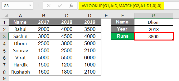
- After applying the Formula, the result is shown below.
- Here if we study the formula, we can see that our data is dependant on two data; in our case, what we write in G1 and G2, in the Match function, we have to select the Column Headers, any of the headers have to be written in G2 which is dedicated to the column name.
- In column G1, we have to write the data from the Row of the Players Name.
- The formula becomes as follows:
=vlookup(G1, A:D, MATCH(G2, A1:D1,0),0)
- Here in the given formula, MATCH(G2, A1:D1,0) is selected column headers cell G2 has to be filled by one of the headers from the selected column header.
- It returns that Dhoni has scored 3800 Runs in 2018.


Comments
Post a Comment